Math Model
Model Justification:
This project will use the numerical technique known as finite difference. This methodology approximates a solution to the governing flow equation by transforming it into a set of algebraic equations with N equations and N unknowns. To solve these large number of algebraic equations we solve iteratively or with direct matrix methods with the aid of computers. Prior to modern computer technology, these approximation methods were not used because of the computational intensity of the methodology. Analytical solutions give you an exact solution, but many times the aquifer and hydraulic assumptions are very restrictive. Numerical solutions (e.g. finite difference) provide a solution with much less restrictive assumptions but do represent an approximation of the actual solution. Using the finite difference approach one will find that the approximation of the solution can only be at discrete locations within the aquifer systems and is subject to round-off and system errors in the solution methodology. But now that computing technology is to a advanced stage, these numerical methods have become the dominant way to mathematically model groundwater flow through the subsurface.When using a numerical methodology, the solutions only determine the dependent variable, which in our cse is the hydraulic head at certain locations. In this project will limit our need to know the hydraulic head to N discret locations, so we will be able to use the Laplace equation in terms of N algebraic equations with N unknown head values.
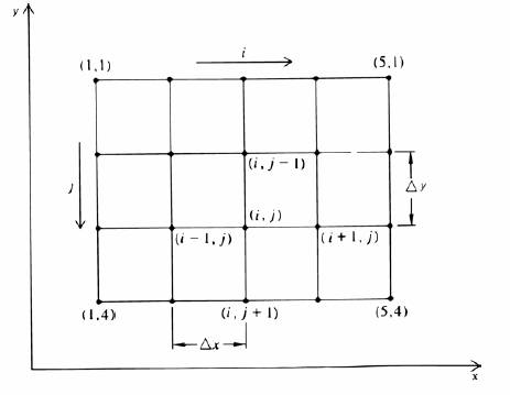
To be able to solve the Laplace equation we will use a grid that will be placed over the flow domain (see figure below)
When the Laplace equation is simplified, one is able to use the following
equation:

Following the above equation, the value of hi,j at any point in the flow is just the average of the head value from its four nearest neighbors in the nodal grid