We have run many simulations after we finished the coding and have obtained many interesting results.
Homogeneous Simulations:
As observed experimentally, for low concentrations, chemicals tend to rearrange themselves into quantum dots. This qualitatively agrees with our simulations as shown in Figure 6A. This simulation starts with low concentrations: C1 = 0.15 and C2 = 0.1. A total scaled time of 0.1 has elapsed in this simulation. Figure 6A shows a nice array of quantum dots with diameters of approximately 3 nm.
As the concentrations of both components increase, the quantum dots become serpentine stripes in Figure 6B. The initial concentrations used in this simulation are C1 = 0.25 and C2 = 0.15. A total scaled time of 0.1 has elapsed.
As the concentrations continue to increase, the serpentine stripes are replaced by quantum pits, which are the opposite of quantum dots (see Figure 6C). For this simulation, C1 = 0.4 and C2 = 0.35. Again, a total scaled time of 0.1 has elapsed. These transitions from quantum dots to serpentine stripes, and to quantum pits, agree qualitatively with experimental observation in Figure 1.
Heterogeneous Simulations:
Heterogeneous simulations have a much wider range of results compared to the homogeneous simulations. For each initial pattern, there is a different result. Thus, heterogeneous simulations are more interesting to study. See Appendix B for more simulations.
The initial pattern of Figure 7A was a circle of concentration .2 to .25. Outside the circle, the concentration was 0.05. This image was taken after a total scaled time of 1 elapsed. The interesting part of simulation is that it originally formed several rings before quantum dots appeared. If we were to run this simulation even longer, all of the rings would become quantum dots arranged in circles. The ring formation is analogous to the ripples created by dropping a rock in water.
Initially in Figure 7B, half of the simulation square had a concentration of 0.3 to 0.35. The other half had a concentration of 0.05. First, a high concentration stripe formed at the boundary. Gradually over time, more stripes formed. Not much happened to the lower concentration aside from the slight increase caused by the higher concentration spreading out. The formation of the stripes was expected. In this simulation, a total time of 0.9 elapsed.
The initial pattern in Figure 7C was a square of concentration 0.4 to 0.45. A total scaled time of 0.9 elapsed. This simulation was not anything like the circle. One might expected it to spread out like the circle. This likely didn’t happen due to the configuration (e.g. the sharp edges). Comparing the simulations of a square, a pentagon, and a circle, we can infer that as the number of sides on the polygon increases, the closer the simulation mimics the circle (it spreads out and forms rings), which makes sense.
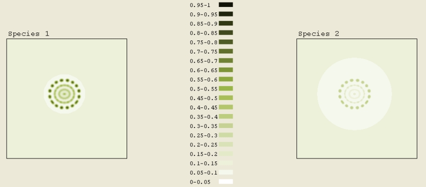
Figure 7A
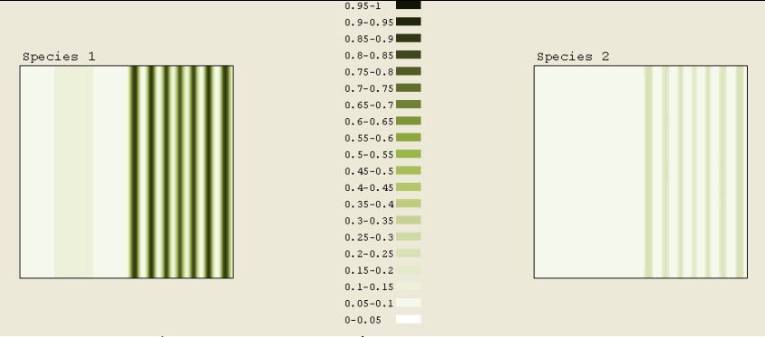
Figure 7B
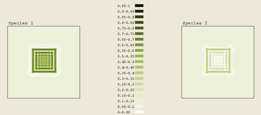
Figure 7C
Figure 8A
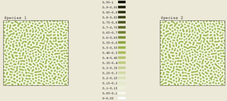
Figure 8B
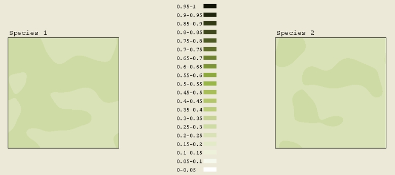
Figure 8C